6.4 이웃 샘플러 커스터마이징하기
DGL이 여러 이웃 샘플링 방법들을 제공하지만, 샘플링 방법을 직접 만들어야할 경우도 있다. 이 절에서는 샘플링 방법을 직접 만드는 방법과 stochastic GNN 학습 프레임워크에서 사용하는 방법을 설명한다.
그래프 뉴럴 네트워크가 얼마나 강력한가(How Powerful are Graph Neural Networks) 에서 설명했듯이, 메시지 전달은 다음과 같이 정의된다.
여기서, \(\rho^{(l)}\) 와 \(\phi^{(l)}\) 는 파라메터를 갖는 함수이고, \(\mathcal{N}(v)`는 그래프 :math:\)mathcal{G}` 에 속한 노드 \(v\) 의 선행 노드(predecessor)들 (또는 방향성 그래프의 경우 이웃 노드들)의 집합을 의미한다.
아래 그래프의 빨간색 노드를 업데이트하는 메시지 전달을 수행하기 위해서는,
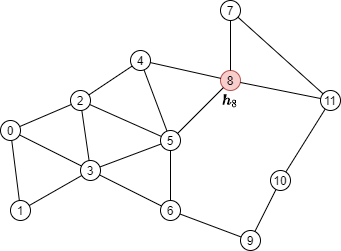
아래 그림의 녹색으로 표시된 이웃 노드들의 노드 피쳐들을 합쳐야한다(aggregate).
이웃 샘플링 직접 해보기
우선 위 그림의 그래프를 DGL 그래프로 정의한다.
import torch
import dgl

src = torch.LongTensor(
    [0, 0, 0, 1, 2, 2, 2, 3, 3, 4, 4, 5, 5, 6, 7, 7, 8, 9, 10,
     1, 2, 3, 3, 3, 4, 5, 5, 6, 5, 8, 6, 8, 9, 8, 11, 11, 10, 11])
dst = torch.LongTensor(
    [1, 2, 3, 3, 3, 4, 5, 5, 6, 5, 8, 6, 8, 9, 8, 11, 11, 10, 11,
     0, 0, 0, 1, 2, 2, 2, 3, 3, 4, 4, 5, 5, 6, 7, 7, 8, 9, 10])
g = dgl.graph((src, dst))
그리고 노드 한개에 대한 결과를 계산하기 위해서 멀티-레이어 메시지 전달을 어떻게 수행할지를 고려하자.
메시지 전달 의존성 찾기
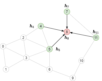
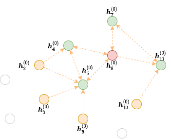
아래 그래프에서 2-레이어 GNN을 사용해서 시드 노드 8의 결과를 계산하는 것을 생각해보자.

공식은 다음과 같다.
이 공식에 따르면, \(\boldsymbol{h}_8^{(2)}\) 을 계산하기 위해서는 아래 그림에서와 같이 (녹색으로 표시된) 노드 4,5,7 그리고 11번에서 에지을 따라서 메시지를 수집하는 것이 필요하다.
이 그래프는 원본 그래프의 모든 노드들을 포함하고 있지만, 특정 출력 노드들에 메시지를 전달할 에지들만을 포함하고 있다. 이런 그래프를 빨간색 노드 8에 대한 두번째 GNN 레이어에 대한 프론티어(frontier) 라고 부른다.
프론티어들을 생성하는데 여러 함수들이 사용된다. 예를 들어, dgl.in_subgraph() 는 원본 그래프의 모든 노드를 포함하지만, 특정 노드의 진입 에지(incoming edge)들만 포함하는 서브 그래프를 유도하는 함수이다.
frontier = dgl.in_subgraph(g, [8])
print(frontier.all_edges())
전체 구현은 Subgraph Extraction Ops 와 dgl.sampling 를 참고하자.
기술적으로는 원본 그래프와 같은 노들들 집합을 잡는 어떤 그래프도 프로티어가 될 수 있다. 이는 커스텀 이웃 샘플러 구현하기 에 대한 기반이다.
멀티-레이어 미니배치 메시지 전달을 위한 이분 구조(Bipartite Structure)
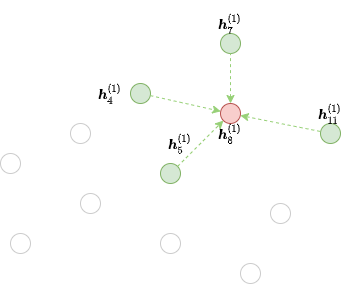
하지만, \(\boldsymbol{h}_\cdot^{(1)}\) 로부터 단순히 \(\boldsymbol{h}_8^{(2)}\) 를 계산하는 것은 프론티어에서 메시지 전달을 계산하는 방식으로 할 수 없다. 그 이유는, 여전히 프론티어가 원본 그래프의 모든 노드를 포함하고 있기 때문이다. 이 그래프의 경우, (녹색과 빨간색 노드들) 4, 5, 7, 8, 11 노드들만이 입력으로 필요하고, 출력으로는 (빨간색 노드) 노드 8번이 필요하다. 입력과 출력의 노드 개수가 다르기 때문에, 작은 이분-구조(bipartite-structured) 그래프에서 메시지 전달을 수행할 필요가 있다.
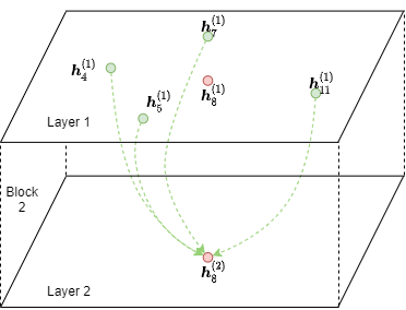
아래 그림은 노드 8에 대해서 2번째 GNN 레이어의 MFG를 보여준다.
Note
Message Flow Graph에 대한 개념은 Stochastic Training Tutorial 참고하자.
목적지 노드들이 소스 노드에도 등장한다는 점을 유의하자. 그 이유는 메시지 전달(예를 들어, \(\phi^{(2)}\) )이 수행된 후에 이전 레이어의 목적지 노드들의 representation들이 피처를 합치는데 사용되기 때문이다.
DGL은 임의의 프론티어를 MFG로 변환하는 dgl.to_block() 함수를 제공한다. 이 함수의 첫번째 인자는 프론티어이고, 두번째 인자는 목적지 노드들이다. 예를 들어, 위 프론티어는 목적지 노드 8에 대한 MFG로 전환하는 코드는 다음과 같다.
dst_nodes = torch.LongTensor([8])
block = dgl.to_block(frontier, dst_nodes)
dgl.DGLGraph.number_of_src_nodes() 와
dgl.DGLGraph.number_of_dst_nodes() 메소스들 사용해서 특정 노트 타입의 소스 노드 및 목적지 노드의 수를 알아낼 수 있다.
num_src_nodes, num_dst_nodes = block.number_of_src_nodes(), block.number_of_dst_nodes()
print(num_src_nodes, num_dst_nodes)
dgl.DGLGraph.srcdata 와 dgl.DGLGraph.srcnodes 같은 멤머를 통해서 MFG의 소스 노드 피쳐들을 접근할 수 있고, dgl.DGLGraph.dstdata 와 dgl.DGLGraph.dstnodes 를 통해서는 목적지 노드의 피쳐들을 접근할 수 있다. srcdata / dstdata 와 srcnodes / dstnodes 의 사용법은 일반 그래프에 사용하는 dgl.DGLGraph.ndata 와 dgl.DGLGraph.nodes 와 동일하다.
block.srcdata['h'] = torch.randn(num_src_nodes, 5)
block.dstdata['h'] = torch.randn(num_dst_nodes, 5)
만약 MFG가 프론티어에서 만들어졌다면, 즉 프래프에서 만들어졌다면, MFG의 소스 및 목적지 노드의 피쳐는 다음과 같이 직접 읽을 수 있다.
print(block.srcdata['x'])
print(block.dstdata['y'])
Note
MFG에서의 소스 노드와 목적지 노드의 원본의 노드 ID는 dgl.NID 피쳐에 저장되어 있고, MFG의 에지 ID들와 프론티어의 에지 ID 사이의 매핑은 dgl.EID 에 있다.
DGL에서는 MFG의 목적지 노드들이 항상 소스 노드에도 있도록 하고 있다. 다음 코드에서 알수 있듯이, 목적지 노드들은 소스 노드들에서 늘 먼저 위치한다.
src_nodes = block.srcdata[dgl.NID]
dst_nodes = block.dstdata[dgl.NID]
assert torch.equal(src_nodes[:len(dst_nodes)], dst_nodes)
그 결과, 목적지 노드들은 프론티어의 에지들의 목적지인 모든 노들들을 포함해야 한다.
예를 들어, 아래 프론티어를 생각해 보자.
여기서 빨간 노드와 녹색 노드들 (즉, 4, 5, 7, 8 그리고 11번 노드)는 에지의 목적지가 되는 노드들이다. 이 경우, 아래 코드는 에러를 발생시키는데, 이유는 목적지 노드 목록이 이들 노드를 모두 포함하지 않기 때문이다.
dgl.to_block(frontier2, torch.LongTensor([4, 5])) # ERROR
하지만, 목적지 노드들은 위 보다 더 많은 노드들을 포함할 수 있다. 이 예제의 경우, 어떤 에지도 연결되지 않은 고립된 노드들(isolated node)이 있고, 이 고립 노드들은 소스 노드와 목적지 노드 모두에 포함될 수 있다.
# Node 3 is an isolated node that do not have any edge pointing to it.
block3 = dgl.to_block(frontier2, torch.LongTensor([4, 5, 7, 8, 11, 3]))
print(block3.srcdata[dgl.NID])
print(block3.dstdata[dgl.NID])
Heterogeneous 그래프들
MFG들은 heterogeneous 그래프에도 적용됩니다. 다음 프론티어를 예로 들어보자.
hetero_frontier = dgl.heterograph({
    ('user', 'follow', 'user'): ([1, 3, 7], [3, 6, 8]),
    ('user', 'play', 'game'): ([5, 5, 4], [6, 6, 2]),
    ('game', 'played-by', 'user'): ([2], [6])
}, num_nodes_dict={'user': 10, 'game': 10})
목적지 노드들 User #3, #4, #8 그리고 Game #2, #6을 포함한 MFG를 생성한다.
hetero_block = dgl.to_block(hetero_frontier, {'user': [3, 6, 8], 'game': [2, 6]})
소스 노드들과 목적지 노드들의 타입별로 얻을 수 있다.
# source users and games
print(hetero_block.srcnodes['user'].data[dgl.NID], hetero_block.srcnodes['game'].data[dgl.NID])
# destination users and games
print(hetero_block.dstnodes['user'].data[dgl.NID], hetero_block.dstnodes['game'].data[dgl.NID])
커스텀 이웃 샘플러 구현하기
아래 코드는 노드 분류를 위한 이웃 샘플링을 수행한다는 것을 떠올려 보자.
sampler = dgl.dataloading.MultiLayerFullNeighborSampler(2)
이웃 샘플링 전략을 직접 구현하기 위해서는 sampler 를 직접 구현한 내용으로 바꾸기만 하면 된다. 이를 살펴보기 위해서, 우선 MultiLayerFullNeighborSampler 를 상속한 클래스인 BlockSampler 를 살펴보자.
BlockSampler 클래스는 sample_blocks() 메소드를 통해서 마지막 레이어로부터 시작하는 MFG들의 리스트를 만들어내는 역할을 한다. sample_blocks 의 기본 구현은 프론티어들과 그것들을 MFG들로 변환하면서 backwards를 iterate한다.
따라서, 이웃 샘플링을 하기 위해서 단지 sample_frontier() 메소드 를 구현하기만 하면된다. 어떤 레이어를 위한 프론티어를 생성할 것인지, 원본 그래프, representation들을 계산할 노드들이 주어지면, 이 메소드는 그것들을 위한 프론티어를 생성하는것을 담당한다.
GNN 레이어 수를 상위 클래스에 전달해야 한다.
예를 들어, MultiLayerFullNeighborSampler 구현은 다음과 같다.
class MultiLayerFullNeighborSampler(dgl.dataloading.BlockSampler):
    def __init__(self, n_layers):
        super().__init__(n_layers)

    def sample_frontier(self, block_id, g, seed_nodes):
        frontier = dgl.in_subgraph(g, seed_nodes)
        return frontier
dgl.dataloading.neighbor.MultiLayerNeighborSampler 는 더 복잡한 이웃 샘플러로, 각 노들에 대해서 메시지를 수집할 적은 수의 이웃 노드들을 샘플하는 기능을 하는데, 구현은 다음과 같다.
class MultiLayerNeighborSampler(dgl.dataloading.BlockSampler):
    def __init__(self, fanouts):
        super().__init__(len(fanouts))

        self.fanouts = fanouts

    def sample_frontier(self, block_id, g, seed_nodes):
        fanout = self.fanouts[block_id]
        if fanout is None:
            frontier = dgl.in_subgraph(g, seed_nodes)
        else:
            frontier = dgl.sampling.sample_neighbors(g, seed_nodes, fanout)
        return frontier
위의 함수는 프론티어를 생성하지만, 원본 그래프와 같은 노들을 갖는 어떤 그래프도 프론티어로 사용될 수 있다.
예를 들어, 주어진 확률에 따라서 시드 노드들에 연결되는 인바운드 에지를 임의로 삭제하기를 원한다면, 다음과 같이 샘플러를 정의할 수 있다.
class MultiLayerDropoutSampler(dgl.dataloading.BlockSampler):
    def __init__(self, p, num_layers):
        super().__init__(num_layers)

        self.p = p

    def sample_frontier(self, block_id, g, seed_nodes, *args, **kwargs):
        # Get all inbound edges to `seed_nodes`
        src, dst = dgl.in_subgraph(g, seed_nodes).all_edges()
        # Randomly select edges with a probability of p
        mask = torch.zeros_like(src).bernoulli_(self.p)
        src = src[mask]
        dst = dst[mask]
        # Return a new graph with the same nodes as the original graph as a
        # frontier
        frontier = dgl.graph((src, dst), num_nodes=g.num_nodes())
        return frontier

    def __len__(self):
        return self.num_layers
샘플러를 직접 구현한 다음에는, 그 샘플러를 사용하는 데이터 로더를 생성하고, 예전과 같이 시드 노드들을 iterate하면서 MFG들의 리스트를 만들게 한다.
sampler = MultiLayerDropoutSampler(0.5, 2)
dataloader = dgl.dataloading.NodeDataLoader(
    g, train_nids, sampler,
    batch_size=1024,
    shuffle=True,
    drop_last=False,
    num_workers=4)

model = StochasticTwoLayerRGCN(in_features, hidden_features, out_features)
model = model.cuda()
opt = torch.optim.Adam(model.parameters())

for input_nodes, blocks in dataloader:
    blocks = [b.to(torch.device('cuda')) for b in blocks]
    input_features = blocks[0].srcdata     # returns a dict
    output_labels = blocks[-1].dstdata     # returns a dict
    output_predictions = model(blocks, input_features)
    loss = compute_loss(output_labels, output_predictions)
    opt.zero_grad()
    loss.backward()
    opt.step()
Heterogeneous 그래프들
Heterogeneous 그래프에 대한 프론티어를 생성하는 것은 homogeneous 그래프의 경우와 동일하다. 리턴된 그래프가 원본 그래프와 같은 노드들을 갖도록 하면, 나머지는 그대로 동작할 것이다. 예를 들어, 위 MultiLayerDropoutSampler 를 재작성해서 모든 에지 타입들을 iterate 해서, heterogeneous 그래프에도 작동하게 만들 수 있다.
class MultiLayerDropoutSampler(dgl.dataloading.BlockSampler):
    def __init__(self, p, num_layers):
        super().__init__(num_layers)

        self.p = p

    def sample_frontier(self, block_id, g, seed_nodes, *args, **kwargs):
        # Get all inbound edges to `seed_nodes`
        sg = dgl.in_subgraph(g, seed_nodes)

        new_edges_masks = {}
        # Iterate over all edge types
        for etype in sg.canonical_etypes:
            edge_mask = torch.zeros(sg.num_edges(etype))
            edge_mask.bernoulli_(self.p)
            new_edges_masks[etype] = edge_mask.bool()

        # Return a new graph with the same nodes as the original graph as a
        # frontier
        frontier = dgl.edge_subgraph(new_edges_masks, relabel_nodes=False)
        return frontier

    def __len__(self):
        return self.num_layers