DGL at a Glance

Author: Minjie Wang, Quan Gan, Jake Zhao, Zheng Zhang

DGL is a Python package dedicated to deep learning on graphs, built atop existing tensor DL frameworks (e.g. Pytorch, MXNet) and simplifying the implementation of graph-based neural networks.

The goal of this tutorial:

• Understand how DGL enables computation on graph from a high level.
• Train a simple graph neural network in DGL to classify nodes in a graph.

At the end of this tutorial, we hope you get a brief feeling of how DGL works.

This tutorial assumes basic familiarity with pytorch.

Step 0: Problem description

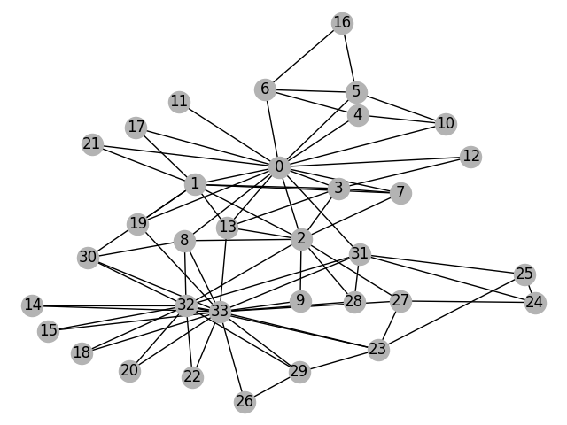
We start with the well-known “Zachary’s karate club” problem. The karate club is a social network which captures 34 members and document pairwise links between members who interact outside the club. The club later divides into two communities led by the instructor (node 0) and the club president (node 33). The network is visualized as follows with the color indicating the community:

The task is to predict which side (0 or 33) each member tends to join given the social network itself.

Step 1: Creating a graph in DGL

Creating the graph for Zachary’s karate club goes as follows:

import dgl

def build_karate_club_graph():
    g = dgl.DGLGraph()
    # add 34 nodes into the graph; nodes are labeled from 0~33
    g.add_nodes(34)
    # all 78 edges as a list of tuples
    edge_list = [(1, 0), (2, 0), (2, 1), (3, 0), (3, 1), (3, 2),
        (4, 0), (5, 0), (6, 0), (6, 4), (6, 5), (7, 0), (7, 1),
        (7, 2), (7, 3), (8, 0), (8, 2), (9, 2), (10, 0), (10, 4),
        (10, 5), (11, 0), (12, 0), (12, 3), (13, 0), (13, 1), (13, 2),
        (13, 3), (16, 5), (16, 6), (17, 0), (17, 1), (19, 0), (19, 1),
        (21, 0), (21, 1), (25, 23), (25, 24), (27, 2), (27, 23),
        (27, 24), (28, 2), (29, 23), (29, 26), (30, 1), (30, 8),
        (31, 0), (31, 24), (31, 25), (31, 28), (32, 2), (32, 8),
        (32, 14), (32, 15), (32, 18), (32, 20), (32, 22), (32, 23),
        (32, 29), (32, 30), (32, 31), (33, 8), (33, 9), (33, 13),
        (33, 14), (33, 15), (33, 18), (33, 19), (33, 20), (33, 22),
        (33, 23), (33, 26), (33, 27), (33, 28), (33, 29), (33, 30),
        (33, 31), (33, 32)]
    # add edges two lists of nodes: src and dst
    src, dst = tuple(zip(*edge_list))
    g.add_edges(src, dst)
    # edges are directional in DGL; make them bi-directional
    g.add_edges(dst, src)

    return g

We can print out the number of nodes and edges in our newly constructed graph:

G = build_karate_club_graph()
print('We have %d nodes.' % G.number_of_nodes())
print('We have %d edges.' % G.number_of_edges())

Out:

We have 34 nodes.
We have 156 edges.

We can also visualize the graph by converting it to a networkx graph:

import networkx as nx
# Since the actual graph is undirected, we convert it for visualization
# purpose.
nx_G = G.to_networkx().to_undirected()
# Kamada-Kawaii layout usually looks pretty for arbitrary graphs
pos = nx.kamada_kawai_layout(nx_G)
nx.draw(nx_G, pos, with_labels=True, node_color=[[.7, .7, .7]])

Step 2: assign features to nodes or edges

Graph neural networks associate features with nodes and edges for training. For our classification example, we assign each node’s an input feature as a one-hot vector: node \(v_i\)‘s feature vector is \([0,\ldots,1,\dots,0]\), where the \(i^{th}\) position is one.

In DGL, we can add features for all nodes at once, using a feature tensor that batches node features along the first dimension. This code below adds the one-hot feature for all nodes:

import torch

G.ndata['feat'] = torch.eye(34)

We can print out the node features to verify:

# print out node 2's input feature
print(G.nodes[2].data['feat'])

# print out node 10 and 11's input features
print(G.nodes[[10, 11]].data['feat'])

Out:

tensor([[0., 0., 1., 0., 0., 0., 0., 0., 0., 0., 0., 0., 0., 0., 0., 0., 0., 0.,
         0., 0., 0., 0., 0., 0., 0., 0., 0., 0., 0., 0., 0., 0., 0., 0.]])
tensor([[0., 0., 0., 0., 0., 0., 0., 0., 0., 0., 1., 0., 0., 0., 0., 0., 0., 0.,
         0., 0., 0., 0., 0., 0., 0., 0., 0., 0., 0., 0., 0., 0., 0., 0.],
        [0., 0., 0., 0., 0., 0., 0., 0., 0., 0., 0., 1., 0., 0., 0., 0., 0., 0.,
         0., 0., 0., 0., 0., 0., 0., 0., 0., 0., 0., 0., 0., 0., 0., 0.]])

Step 3: define a Graph Convolutional Network (GCN)

To perform node classification, we use the Graph Convolutional Network (GCN) developed by Kipf and Welling. Here we provide the simplest definition of a GCN framework, but we recommend the reader to read the original paper for more details.

• At layer \(l\), each node \(v_i^l\) carries a feature vector \(h_i^l\).
• Each layer of the GCN tries to aggregate the features from \(u_i^{l}\) where \(u_i\)‘s are neighborhood nodes to \(v\) into the next layer representation at \(v_i^{l+1}\). This is followed by an affine transformation with some non-linearity.

The above definition of GCN fits into a message-passing paradigm: each node will update its own feature with information sent from neighboring nodes. A graphical demonstration is displayed below.

Now, we show that the GCN layer can be easily implemented in DGL.

import torch.nn as nn
import torch.nn.functional as F

# Define the message & reduce function
# NOTE: we ignore the GCN's normalization constant c_ij for this tutorial.
def gcn_message(edges):
    # The argument is a batch of edges.
    # This computes a (batch of) message called 'msg' using the source node's feature 'h'.
    return {'msg' : edges.src['h']}

def gcn_reduce(nodes):
    # The argument is a batch of nodes.
    # This computes the new 'h' features by summing received 'msg' in each node's mailbox.
    return {'h' : torch.sum(nodes.mailbox['msg'], dim=1)}

# Define the GCNLayer module
class GCNLayer(nn.Module):
    def __init__(self, in_feats, out_feats):
        super(GCNLayer, self).__init__()
        self.linear = nn.Linear(in_feats, out_feats)

    def forward(self, g, inputs):
        # g is the graph and the inputs is the input node features
        # first set the node features
        g.ndata['h'] = inputs
        # trigger message passing on all edges
        g.send(g.edges(), gcn_message)
        # trigger aggregation at all nodes
        g.recv(g.nodes(), gcn_reduce)
        # get the result node features
        h = g.ndata.pop('h')
        # perform linear transformation
        return self.linear(h)

In general, the nodes send information computed via the message functions, and aggregates incoming information with the reduce functions.

We then define a deeper GCN model that contains two GCN layers:

# Define a 2-layer GCN model
class GCN(nn.Module):
    def __init__(self, in_feats, hidden_size, num_classes):
        super(GCN, self).__init__()
        self.gcn1 = GCNLayer(in_feats, hidden_size)
        self.gcn2 = GCNLayer(hidden_size, num_classes)

    def forward(self, g, inputs):
        h = self.gcn1(g, inputs)
        h = torch.relu(h)
        h = self.gcn2(g, h)
        return h
# The first layer transforms input features of size of 34 to a hidden size of 5.
# The second layer transforms the hidden layer and produces output features of
# size 2, corresponding to the two groups of the karate club.
net = GCN(34, 5, 2)

Step 4: data preparation and initialization

We use one-hot vectors to initialize the node features. Since this is a semi-supervised setting, only the instructor (node 0) and the club president (node 33) are assigned labels. The implementation is available as follow.

inputs = torch.eye(34)
labeled_nodes = torch.tensor([0, 33])  # only the instructor and the president nodes are labeled
labels = torch.tensor([0, 1])  # their labels are different

Step 5: train then visualize

The training loop is exactly the same as other PyTorch models. We (1) create an optimizer, (2) feed the inputs to the model, (3) calculate the loss and (4) use autograd to optimize the model.

optimizer = torch.optim.Adam(net.parameters(), lr=0.01)
all_logits = []
for epoch in range(30):
    logits = net(G, inputs)
    # we save the logits for visualization later
    all_logits.append(logits.detach())
    logp = F.log_softmax(logits, 1)
    # we only compute loss for labeled nodes
    loss = F.nll_loss(logp[labeled_nodes], labels)

    optimizer.zero_grad()
    loss.backward()
    optimizer.step()

    print('Epoch %d | Loss: %.4f' % (epoch, loss.item()))

Out:

Epoch 0 | Loss: 2.7260
Epoch 1 | Loss: 2.1398
Epoch 2 | Loss: 1.6107
Epoch 3 | Loss: 1.1329
Epoch 4 | Loss: 0.7571
Epoch 5 | Loss: 0.5086
Epoch 6 | Loss: 0.3634
Epoch 7 | Loss: 0.2876
Epoch 8 | Loss: 0.2486
Epoch 9 | Loss: 0.2241
Epoch 10 | Loss: 0.2022
Epoch 11 | Loss: 0.1826
Epoch 12 | Loss: 0.1631
Epoch 13 | Loss: 0.1418
Epoch 14 | Loss: 0.1209
Epoch 15 | Loss: 0.1015
Epoch 16 | Loss: 0.0841
Epoch 17 | Loss: 0.0690
Epoch 18 | Loss: 0.0554
Epoch 19 | Loss: 0.0442
Epoch 20 | Loss: 0.0352
Epoch 21 | Loss: 0.0279
Epoch 22 | Loss: 0.0222
Epoch 23 | Loss: 0.0177
Epoch 24 | Loss: 0.0141
Epoch 25 | Loss: 0.0113
Epoch 26 | Loss: 0.0090
Epoch 27 | Loss: 0.0074
Epoch 28 | Loss: 0.0061
Epoch 29 | Loss: 0.0051

This is a rather toy example, so it does not even have a validation or test set. Instead, Since the model produces an output feature of size 2 for each node, we can visualize by plotting the output feature in a 2D space. The following code animates the training process from initial guess (where the nodes are not classified correctly at all) to the end (where the nodes are linearly separable).

import matplotlib.animation as animation
import matplotlib.pyplot as plt

def draw(i):
    cls1color = '#00FFFF'
    cls2color = '#FF00FF'
    pos = {}
    colors = []
    for v in range(34):
        pos[v] = all_logits[i][v].numpy()
        cls = pos[v].argmax()
        colors.append(cls1color if cls else cls2color)
    ax.cla()
    ax.axis('off')
    ax.set_title('Epoch: %d' % i)
    nx.draw_networkx(nx_G.to_undirected(), pos, node_color=colors,
            with_labels=True, node_size=300, ax=ax)

fig = plt.figure(dpi=150)
fig.clf()
ax = fig.subplots()
draw(0)  # draw the prediction of the first epoch
plt.close()

The following animation shows how the model correctly predicts the community after a series of training epochs.

ani = animation.FuncAnimation(fig, draw, frames=len(all_logits), interval=200)

Next steps

In the next tutorial, we will go through some more basics of DGL, such as reading and writing node/edge features.

Total running time of the script: ( 0 minutes 0.249 seconds)