Batched Graph Classification with DGL

Author: Mufei Li, Minjie Wang, Zheng Zhang.

Graph classification is an important problem with applications across many fields – bioinformatics, chemoinformatics, social network analysis, urban computing and cyber-security. Applying graph neural networks to this problem has been a popular approach recently ( Ying et al., 2018, Cangea et al., 2018, Knyazev et al., 2018, Bianchi et al., 2019, Liao et al., 2019, Gao et al., 2019).

This tutorial demonstrates:

• batching multiple graphs of variable size and shape with DGL
• training a graph neural network for a simple graph classification task

Simple Graph Classification Task

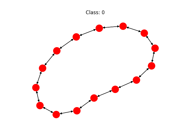
In this tutorial, we will learn how to perform batched graph classification with dgl via a toy example of classifying 8 types of regular graphs as below:

We implement a synthetic dataset data.MiniGCDataset in DGL. The dataset has 8 different types of graphs and each class has the same number of graph samples.

from dgl.data import MiniGCDataset
import matplotlib.pyplot as plt
import networkx as nx
# A dataset with 80 samples, each graph is
# of size [10, 20]
dataset = MiniGCDataset(80, 10, 20)
graph, label = dataset[0]
fig, ax = plt.subplots()
nx.draw(graph.to_networkx(), ax=ax)
ax.set_title('Class: {:d}'.format(label))
plt.show()

Form a graph mini-batch

To train neural networks more efficiently, a common practice is to batch multiple samples together to form a mini-batch. Batching fixed-shaped tensor inputs is quite easy (for example, batching two images of size \(28\times 28\) gives a tensor of shape \(2\times 28\times 28\)). By contrast, batching graph inputs has two challenges:

• Graphs are sparse.
• Graphs can have various length (e.g. number of nodes and edges).

To address this, DGL provides a dgl.batch() API. It leverages the trick that a batch of graphs can be viewed as a large graph that have many disjoint connected components. Below is a visualization that gives the general idea:

We define the following collate function to form a mini-batch from a given list of graph and label pairs.

import dgl

def collate(samples):
    # The input `samples` is a list of pairs
    #  (graph, label).
    graphs, labels = map(list, zip(*samples))
    batched_graph = dgl.batch(graphs)
    return batched_graph, torch.tensor(labels)

The return type of dgl.batch() is still a graph (similar to the fact that a batch of tensors is still a tensor). This means that any code that works for one graph immediately works for a batch of graphs. More importantly, since DGL processes messages on all nodes and edges in parallel, this greatly improves efficiency.

Graph Classifier

The graph classification can be proceeded as follows:

From a batch of graphs, we first perform message passing/graph convolution for nodes to “communicate” with others. After message passing, we compute a tensor for graph representation from node (and edge) attributes. This step may be called “readout/aggregation” interchangeably. Finally, the graph representations can be fed into a classifier \(g\) to predict the graph labels.

Graph Convolution

Our graph convolution operation is basically the same as that for GCN (checkout our tutorial). The only difference is that we replace \(h_{v}^{(l+1)} = \text{ReLU}\left(b^{(l)}+\sum_{u\in\mathcal{N}(v)}h_{u}^{(l)}W^{(l)}\right)\) by \(h_{v}^{(l+1)} = \text{ReLU}\left(b^{(l)}+\frac{1}{|\mathcal{N}(v)|}\sum_{u\in\mathcal{N}(v)}h_{u}^{(l)}W^{(l)}\right)\). The replacement of summation by average is to balance nodes with different degrees, which gives a better performance for this experiment.

Note that the self edges added in the dataset initialization allows us to include the original node feature \(h_{v}^{(l)}\) when taking the average.

import dgl.function as fn
import torch
import torch.nn as nn


# Sends a message of node feature h.
msg = fn.copy_src(src='h', out='m')

def reduce(nodes):
    """Take an average over all neighbor node features hu and use it to
    overwrite the original node feature."""
    accum = torch.mean(nodes.mailbox['m'], 1)
    return {'h': accum}

class NodeApplyModule(nn.Module):
    """Update the node feature hv with ReLU(Whv+b)."""
    def __init__(self, in_feats, out_feats, activation):
        super(NodeApplyModule, self).__init__()
        self.linear = nn.Linear(in_feats, out_feats)
        self.activation = activation

    def forward(self, node):
        h = self.linear(node.data['h'])
        h = self.activation(h)
        return {'h' : h}

class GCN(nn.Module):
    def __init__(self, in_feats, out_feats, activation):
        super(GCN, self).__init__()
        self.apply_mod = NodeApplyModule(in_feats, out_feats, activation)

    def forward(self, g, feature):
        # Initialize the node features with h.
        g.ndata['h'] = feature
        g.update_all(msg, reduce)
        g.apply_nodes(func=self.apply_mod)
        return g.ndata.pop('h')

Readout and Classification

For this demonstration, we consider initial node features to be their degrees. After two rounds of graph convolution, we perform a graph readout by averaging over all node features for each graph in the batch

\[h_g=\frac{1}{|\mathcal{V}|}\sum_{v\in\mathcal{V}}h_{v}\]

In DGL, dgl.mean_nodes() handles this task for a batch of graphs with variable size. We then feed our graph representations into a classifier with one linear layer to obtain pre-softmax logits.

import torch.nn.functional as F


class Classifier(nn.Module):
    def __init__(self, in_dim, hidden_dim, n_classes):
        super(Classifier, self).__init__()

        self.layers = nn.ModuleList([
            GCN(in_dim, hidden_dim, F.relu),
            GCN(hidden_dim, hidden_dim, F.relu)])
        self.classify = nn.Linear(hidden_dim, n_classes)

    def forward(self, g):
        # For undirected graphs, in_degree is the same as
        # out_degree.
        h = g.in_degrees().view(-1, 1).float()
        for conv in self.layers:
            h = conv(g, h)
        g.ndata['h'] = h
        hg = dgl.mean_nodes(g, 'h')
        return self.classify(hg)

Setup and Training

We create a synthetic dataset of \(400\) graphs with \(10\) ~ \(20\) nodes. \(320\) graphs constitute a training set and \(80\) graphs constitute a test set.

import torch.optim as optim
from torch.utils.data import DataLoader

# Create training and test sets.
trainset = MiniGCDataset(320, 10, 20)
testset = MiniGCDataset(80, 10, 20)
# Use PyTorch's DataLoader and the collate function
# defined before.
data_loader = DataLoader(trainset, batch_size=32, shuffle=True,
                         collate_fn=collate)

# Create model
model = Classifier(1, 256, trainset.num_classes)
loss_func = nn.CrossEntropyLoss()
optimizer = optim.Adam(model.parameters(), lr=0.001)
model.train()

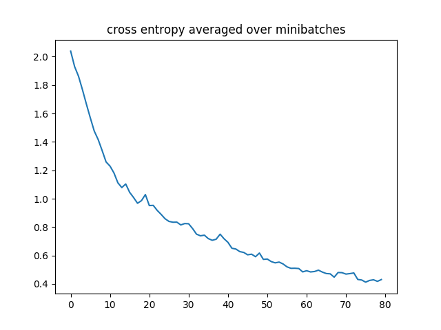
epoch_losses = []
for epoch in range(80):
    epoch_loss = 0
    for iter, (bg, label) in enumerate(data_loader):
        prediction = model(bg)
        loss = loss_func(prediction, label)
        optimizer.zero_grad()
        loss.backward()
        optimizer.step()
        epoch_loss += loss.detach().item()
    epoch_loss /= (iter + 1)
    print('Epoch {}, loss {:.4f}'.format(epoch, epoch_loss))
    epoch_losses.append(epoch_loss)

Out:

Epoch 0, loss 2.0386
Epoch 1, loss 1.9301
Epoch 2, loss 1.8616
Epoch 3, loss 1.7670
Epoch 4, loss 1.6657
Epoch 5, loss 1.5687
Epoch 6, loss 1.4759
Epoch 7, loss 1.4161
Epoch 8, loss 1.3392
Epoch 9, loss 1.2590
Epoch 10, loss 1.2297
Epoch 11, loss 1.1817
Epoch 12, loss 1.1121
Epoch 13, loss 1.0782
Epoch 14, loss 1.1035
Epoch 15, loss 1.0447
Epoch 16, loss 1.0082
Epoch 17, loss 0.9678
Epoch 18, loss 0.9863
Epoch 19, loss 1.0290
Epoch 20, loss 0.9515
Epoch 21, loss 0.9529
Epoch 22, loss 0.9178
Epoch 23, loss 0.8897
Epoch 24, loss 0.8590
Epoch 25, loss 0.8400
Epoch 26, loss 0.8344
Epoch 27, loss 0.8349
Epoch 28, loss 0.8153
Epoch 29, loss 0.8250
Epoch 30, loss 0.8235
Epoch 31, loss 0.7898
Epoch 32, loss 0.7502
Epoch 33, loss 0.7388
Epoch 34, loss 0.7432
Epoch 35, loss 0.7189
Epoch 36, loss 0.7072
Epoch 37, loss 0.7147
Epoch 38, loss 0.7502
Epoch 39, loss 0.7180
Epoch 40, loss 0.6925
Epoch 41, loss 0.6510
Epoch 42, loss 0.6458
Epoch 43, loss 0.6274
Epoch 44, loss 0.6218
Epoch 45, loss 0.6050
Epoch 46, loss 0.6095
Epoch 47, loss 0.5917
Epoch 48, loss 0.6174
Epoch 49, loss 0.5728
Epoch 50, loss 0.5752
Epoch 51, loss 0.5573
Epoch 52, loss 0.5484
Epoch 53, loss 0.5537
Epoch 54, loss 0.5407
Epoch 55, loss 0.5203
Epoch 56, loss 0.5098
Epoch 57, loss 0.5104
Epoch 58, loss 0.5084
Epoch 59, loss 0.4846
Epoch 60, loss 0.4930
Epoch 61, loss 0.4844
Epoch 62, loss 0.4873
Epoch 63, loss 0.4970
Epoch 64, loss 0.4834
Epoch 65, loss 0.4732
Epoch 66, loss 0.4710
Epoch 67, loss 0.4475
Epoch 68, loss 0.4804
Epoch 69, loss 0.4793
Epoch 70, loss 0.4693
Epoch 71, loss 0.4727
Epoch 72, loss 0.4773
Epoch 73, loss 0.4314
Epoch 74, loss 0.4277
Epoch 75, loss 0.4125
Epoch 76, loss 0.4246
Epoch 77, loss 0.4292
Epoch 78, loss 0.4180
Epoch 79, loss 0.4308

The learning curve of a run is presented below:

plt.title('cross entropy averaged over minibatches')
plt.plot(epoch_losses)
plt.show()

The trained model is evaluated on the test set created. Note that for deployment of the tutorial, we restrict our running time and you are likely to get a higher accuracy (\(80\) % ~ \(90\) %) than the ones printed below.

model.eval()
# Convert a list of tuples to two lists
test_X, test_Y = map(list, zip(*testset))
test_bg = dgl.batch(test_X)
test_Y = torch.tensor(test_Y).float().view(-1, 1)
probs_Y = torch.softmax(model(test_bg), 1)
sampled_Y = torch.multinomial(probs_Y, 1)
argmax_Y = torch.max(probs_Y, 1)[1].view(-1, 1)
print('Accuracy of sampled predictions on the test set: {:.4f}%'.format(
    (test_Y == sampled_Y.float()).sum().item() / len(test_Y) * 100))
print('Accuracy of argmax predictions on the test set: {:4f}%'.format(
    (test_Y == argmax_Y.float()).sum().item() / len(test_Y) * 100))

Out:

Accuracy of sampled predictions on the test set: 68.7500%
Accuracy of argmax predictions on the test set: 76.250000%

Below is an animation where we plot graphs with the probability a trained model assigns its ground truth label to it:

To understand the node/graph representations a trained model learnt, we use t-SNE, for dimensionality reduction and visualization.

The two small figures on the top separately visualize node representations after \(1\), \(2\) layers of graph convolution and the figure on the bottom visualizes the pre-softmax logits for graphs as graph representations.

While the visualization does suggest some clustering effects of the node features, it is expected not to be a perfect result as node degrees are deterministic for our node features. Meanwhile, the graph features are way better separated.

What’s Next?

Graph classification with graph neural networks is still a very young field waiting for folks to bring more exciting discoveries! It is not easy as it requires mapping different graphs to different embeddings while preserving their structural similarity in the embedding space. To learn more about it, “How Powerful Are Graph Neural Networks?” in ICLR 2019 might be a good starting point.

With regards to more examples on batched graph processing, see

• our tutorials on Tree LSTM and Deep Generative Models of Graphs
• an example implementation of Junction Tree VAE

Total running time of the script: ( 0 minutes 20.163 seconds)